
I created this on my phone in MATLAB. You can probably do this in Octave with similar or the same code.
First, I downloaded the image from Lemmy, then uploaded it into my MATLAB app. I renamed the image to image.jpg, then ran the following code:
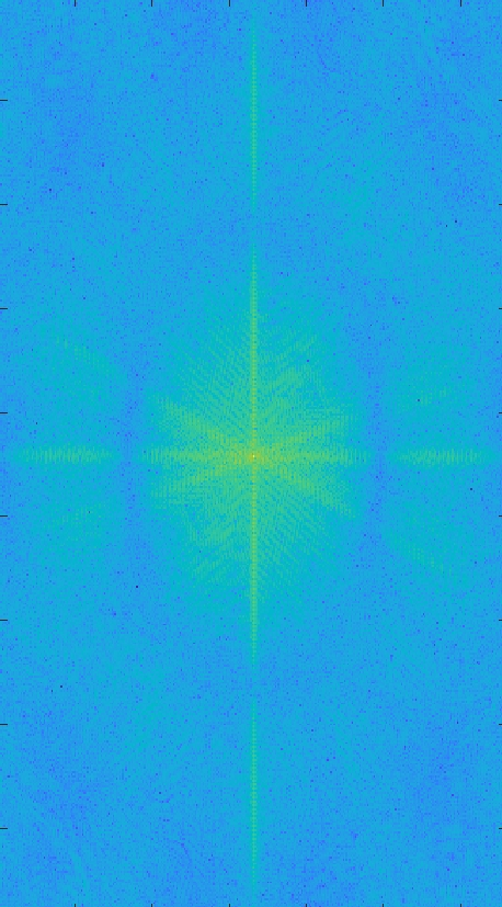
image=imread(“image.jpg”) imagesc(log10(abs( fftshift(fft2(image)) )))
fft2 applies a 2D Fast Fourier transform to the image, which creates a complex (as in complex numbers) image. abs takes the magnitude of the complex image elementwise. log10 scales the result for display.
Then I downloaded the image from the MATLAB app, went into the Photos app and (badly) cropped out the white border.
Despite how dramatically different it looks, it actually contains the same [1] information as the original image. Said differently, you can actually go back to the original with the inverse functions, specifically by undoing the logarithm and applying the inverse FFT.
[1] Almost. (1). There will be border problems potentially caused by me sloppily cropping some pixels out of the image. (2). It looks like MATLAB resized the image when rendering the figure. However, if I actually saved the matrix (raw image) rather than the figure, then it would be the correct size. (3) (Thank you to @itslilith@lemmy.blahaj.zone for pointing this out.) You need the phase information to reconstruct the original signal, which I (intentionally) threw out (to get a real image) when I took the absolute value but then completely forgot about it.
Can guarantee OP didn’t expect this when he was making the post, damn
don’t you lose information by taking the abs(), since to restore the full information you need both complex and imaginary parts of the fft? You could probably get away with encoding Re and Im in different color channels tho
Another nice way one could preserve the complex data when visualizing it would be to make a 3d color mesh and display the imaginary components as the height in z and the real component as the color scale (or vice-versa).
Edit* now I am trying to think if there would be a clever way to show the abs, Re and Im values in one 3d plot, but drawing a blank. Maybe tie Im to the alpha value to make the transparency change as the imaginary component goes up and down? It would just require mapping the set of all numbers from -inf:inf to 0:1, which is doable in a 1-1 transformation iirc since they both have cardinality C. I think it would be
alpha = 1 - 1/(1-e^{Im(z)})
Which looks a lot like the equation for Bose-Einstein statistics in Stat. Mech. I was never very good at complex analysis or group theory though, so I don’t really know what to make of that.
Bose-Einstein isn’t a great fit, since you’d need to integrate, and it only goes from 0:inf. For mapping the reals to 0:1 you could use arctan and shift it a bit.
Now I’m thinking, instead of color and alpha, you could use two out of hue, saturation and value for Re and Im (or all three, and plot Abs as well)
Ah, you’re right, I haven’t taken Stat. Mech. in almost 5 years so my brain just latched on to the general form. Analysis in frequency space is always fun
Correct. I updated my comment.
Apply a nice gaussian kernel convolution to the fft and smooth that doodle out! Lets get blurry up in this doodle party!
Apply a nice gaussian kernel convolution to the fft
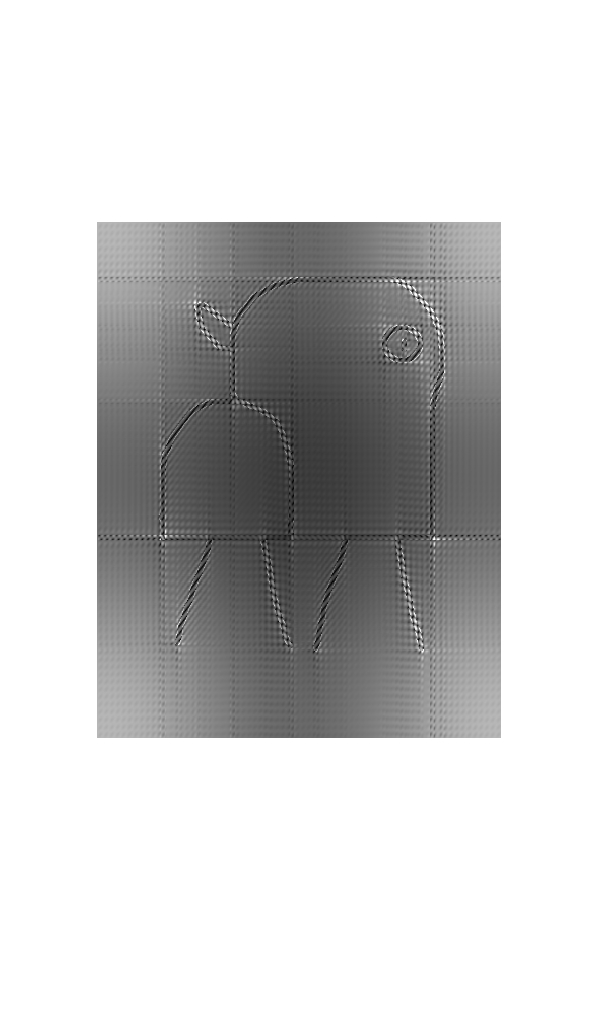
I applied the following code in MATLAB:
new_image = abs(ifft2(conv2(fft2(image),fspecial(‘gaussian’,69)))); imwrite(new_image,“new_image.png”)
And got this:
Oh fuck yeah
Just noticed that you chose the nicest kernel size. Even better.
Ok, this is really mad cool, I like it
Saving this comment in case I ever need a new phone background.
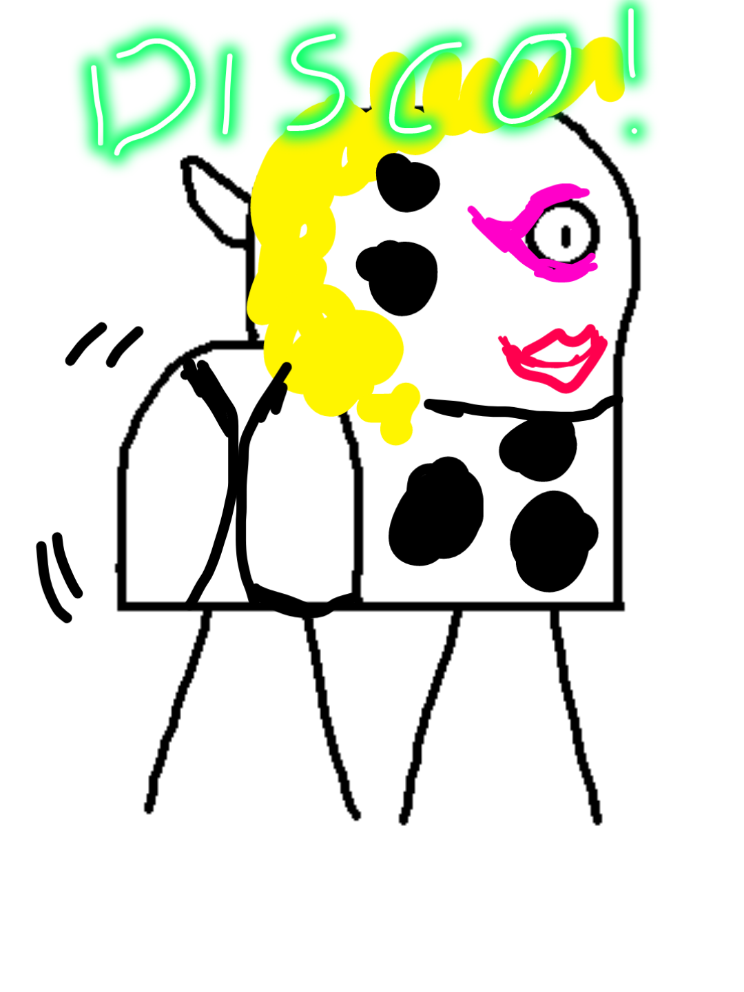
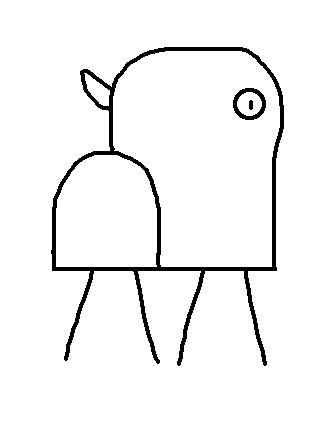
I used the default photos app on my phone to draw a totally normal cow

So I took your image and
ruined my MATLAB accountused the most normal part of your totally normal cow as a 3D [1]cockvolutionconvolution kernel. So in some sense, I dragged the red and purple part all across your image and added up the results. Here’s the result: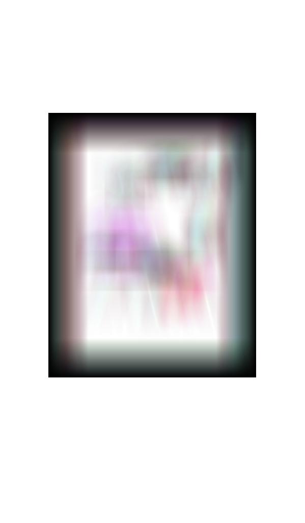
Here’s the MATLAB code:
normal_image = imread(“totally_normal_image.png”);
feature=normal_image(272:350,205:269,:);
feature_expansion = padarray(feature,[0,ceil((79-65)/2),0],‘replicate’);
for m = 1:1:3
new_normal_image(:,:,m) = conv2(normal_image(:,:,m),feature_expansion(:,:,m));

new_normal_image(:,:,m) = new_normal_image(:,:,m)/max(max(new_normal_image(:,:,m)));
end
imshow(new_normal_image)
[1] The original image was practically grayscale, so only a 2D convolution is required, i.e. over 2 spatial dimensions. Since you added color, it adds a extra dimension, one per color channel. Which makes it more annoying to work with in MATLAB. I mean, I could have just dumped everything into grayscale, but I need practice with processing color images anyways.
This is so f’n weird, I love it
Is that supposed to be a blood on the bottom right?
I think it’s a little more nsfw
I mean there’s blood inside the red thing.

over 9000 hours on paint
spoiler
.net
9000 hours well spent
I used an app on my phone to draw over the image and made a cow twerking at the disco.
Oddly specific but ok
I mirrored the image and added scanlines

No, you gave it a dump truck
This could be a logo for a hacker group or a scene group
Lol yeah I can see it working for either of those!
Bulls in Spaaaace!
holly ahit open source drawing
Free and open-source baby, powered by CC BY-NC content license
Hold on this is gonna take some time but I might just try this and post in a few weeks
Now we wait and see what I come up with
I will watch your progress with the great interest
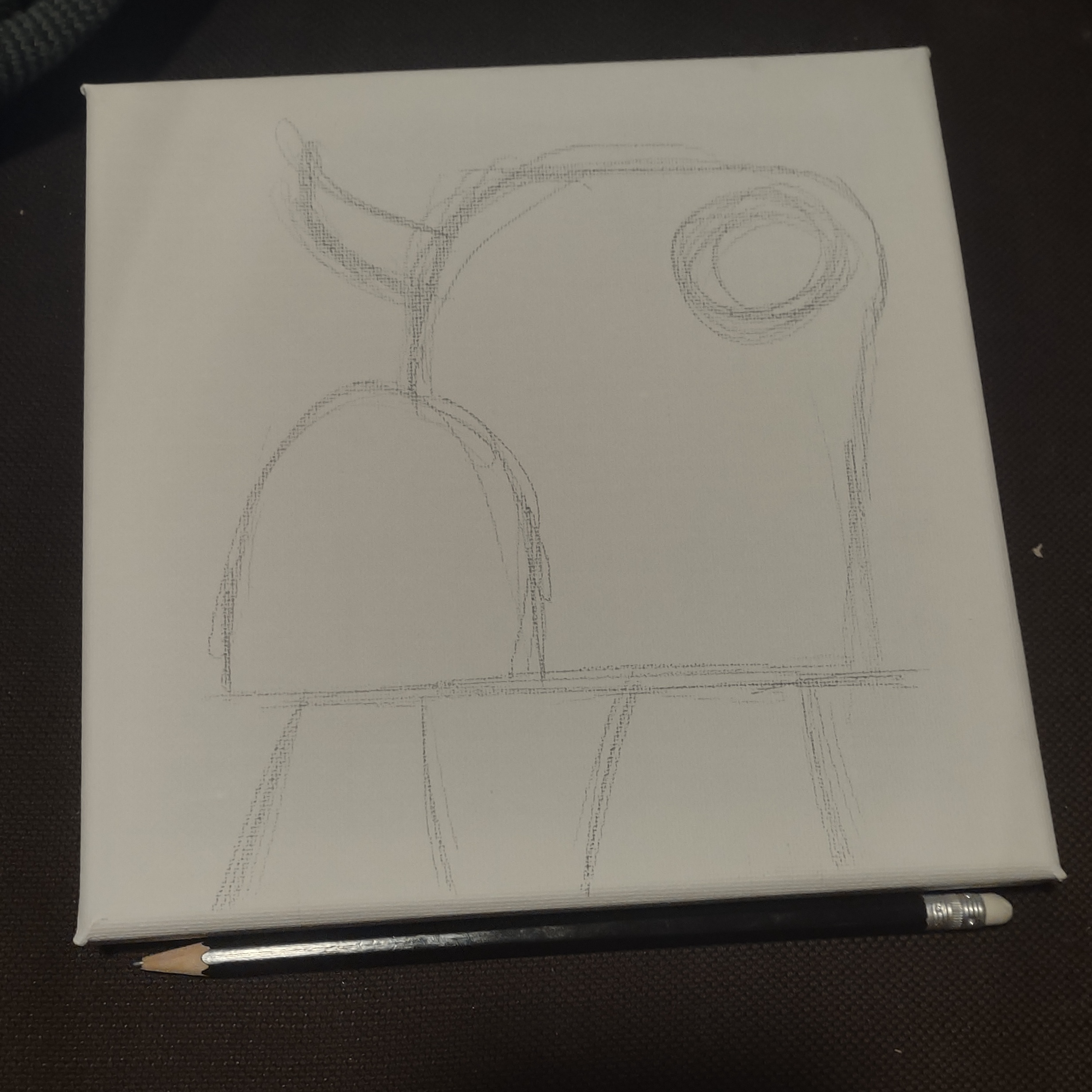
Okay hold on; I did it in a few hours, not weeks but it gets freaky fast:
-
Played around with the lines; erasing a few bits and rounding off some corners.
-
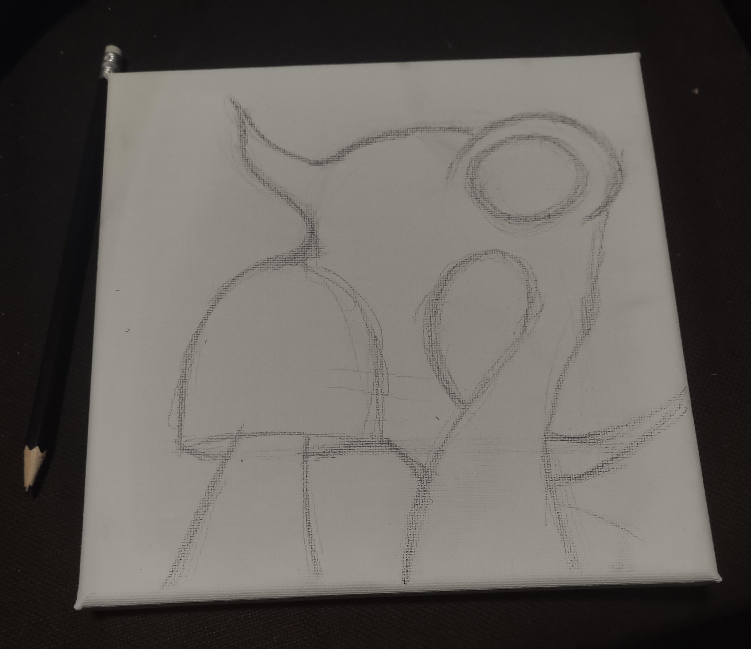
Did the outlines in marker
-
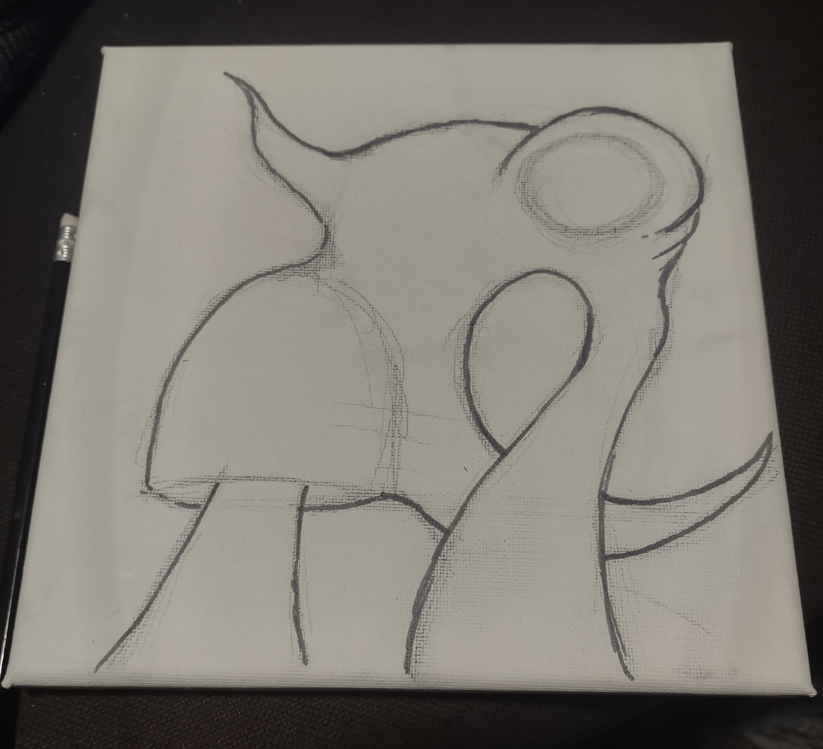
First bit of shading
-
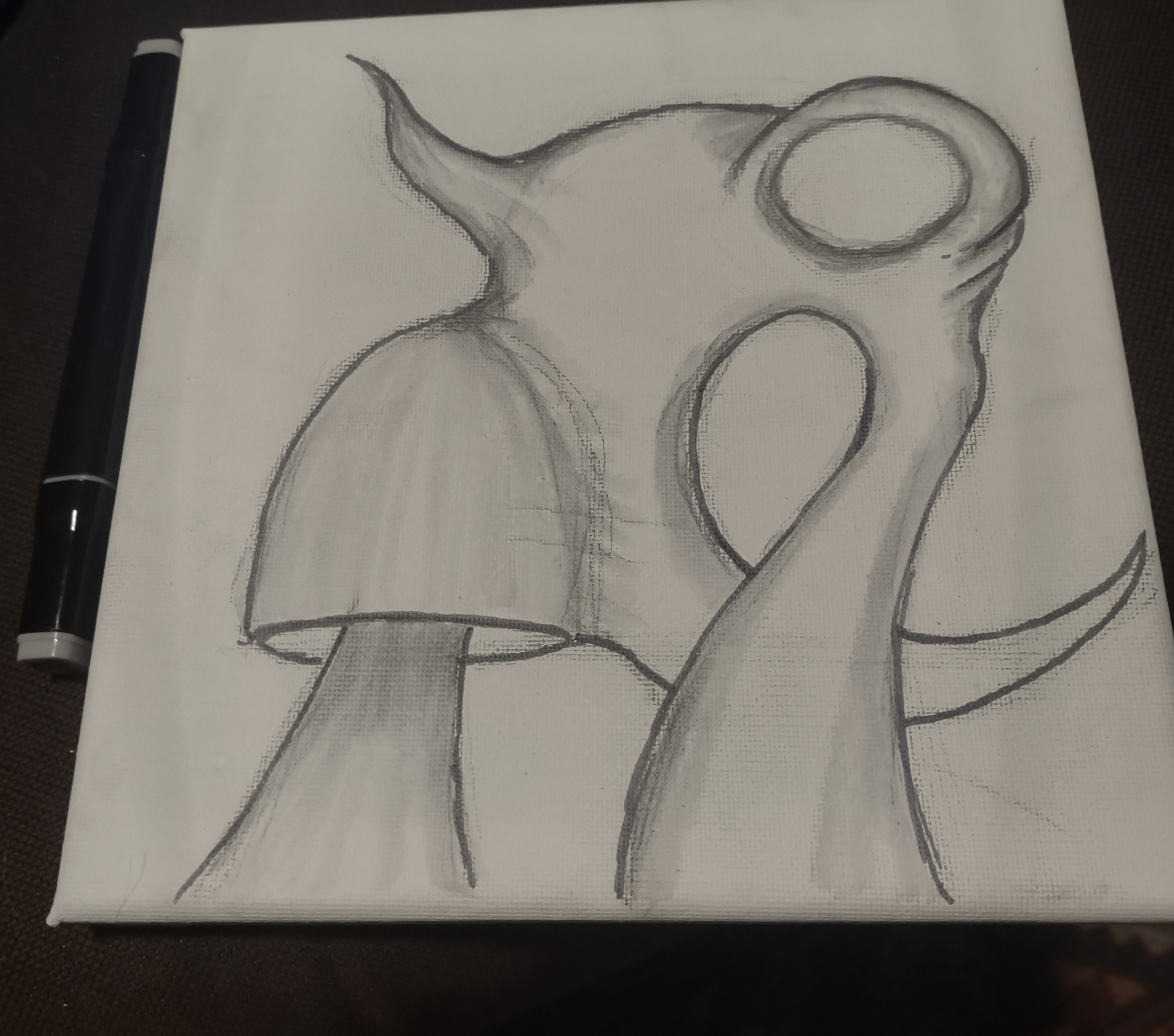
Left it overnight. Came back today and started building up the shades and lines

-
Bit more

-
Bit more and now I think I’m done.
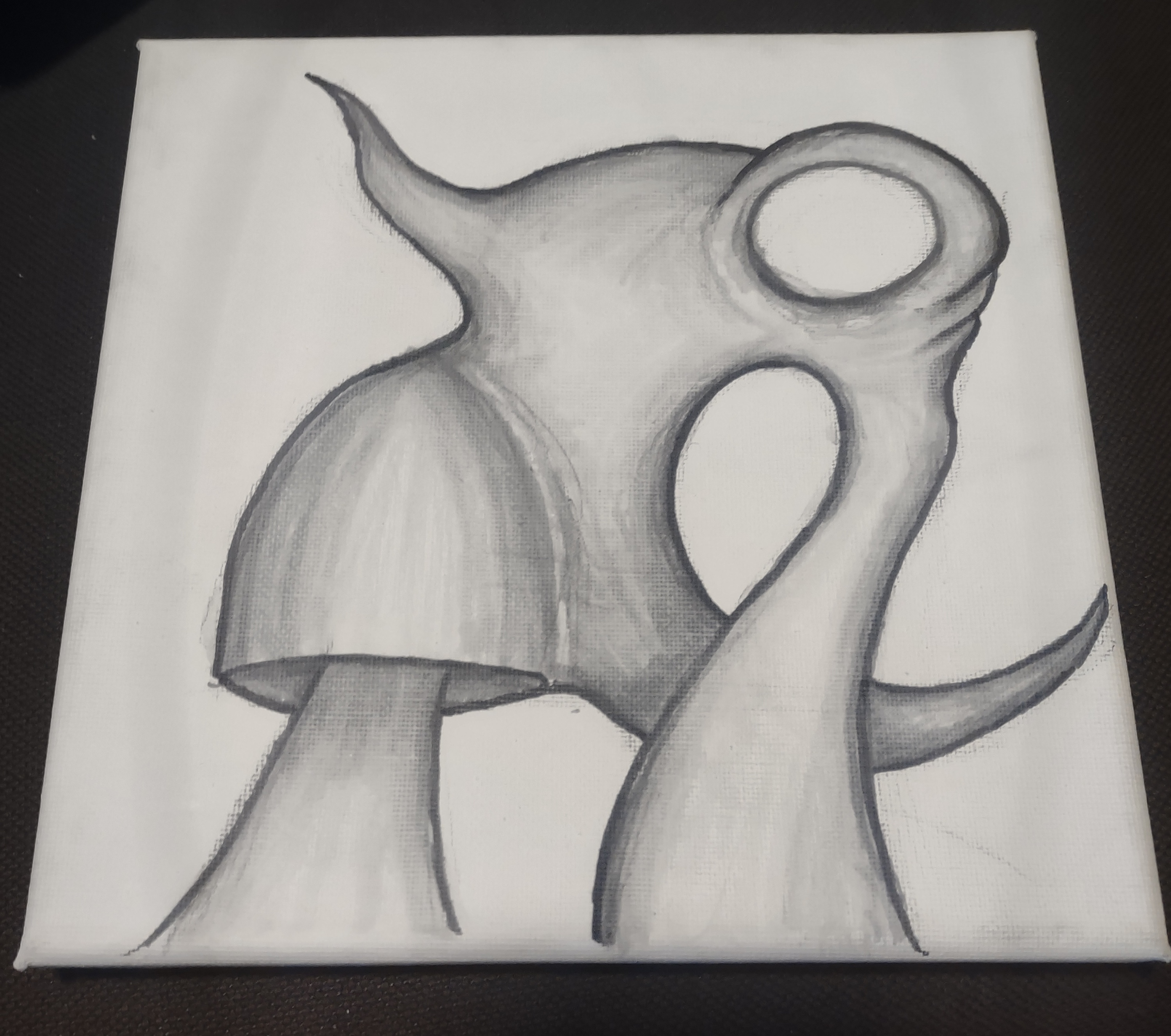
Also my friend asked for a drawing of some mushrooms so I think I’m gonna use the same template for that :)
Can we do these more often? This is fun! :D
What community would fit something like this?
Good question; probably its own?
Looks like a monster for a JRPG, pretty cool and well drawn
-
deleted by creator


